Introduction to Image Processing#
Image processing refers to the analysis, processing, and processing of images to meet visual, psychological, or other requirements. Image processing is an application of signal processing in the field of images. Currently, most images are stored in digital form, so in many cases, image processing refers to digital image processing. In addition, processing methods based on optical theory still occupy an important position.
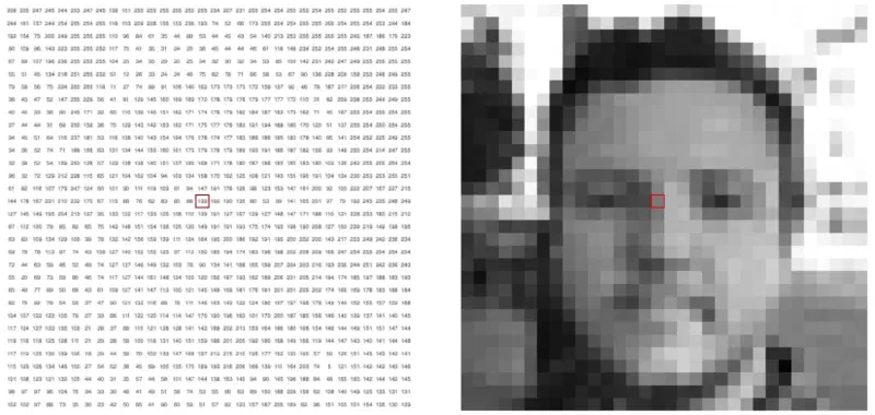
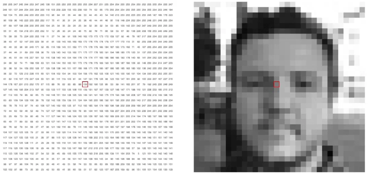
Images in computers are composed of a large number of seemingly continuous pixels, and mathematically, each pixel of an image can correspond to each element of a matrix in linear algebra, so images can be represented using matrices. The types of images vary, and the dimensions of the matrices will change: a grayscale image can be represented by a two-dimensional matrix with element values ranging from 0 to 255, where the element value corresponds to the brightness of the pixel (0 corresponds to black, 255 corresponds to white); a color image (RGB image) can be represented by a three-dimensional matrix, with the red (R), green (G), and blue (B) components represented by three separate matrices, and the combination of the three matrices forms the three-dimensional matrix. It can be said that an image is equivalent to a matrix, so the results of matrix theory in linear algebra can be applied to image processing.

Simple Geometric Transformations#
Treating image information as a matrix for processing, we can utilize the knowledge of matrix theory in linear algebra to perform simple geometric transformations on images. The following introduces several common principles of image geometric transformations, where \(x’\), \(y’\) are the pixel coordinates of the transformed image, \(x_0\), \(y_0\) are the offsets in each direction, and \(x\), \(y\) are the pixel coordinates of the original image.
Translation#
$$ \begin{bmatrix} x’ \cr y’ \cr 1 \end{bmatrix} = \begin{bmatrix} 1&0&x_0\cr 0&1&y_0\cr 0&0&1 \end{bmatrix} \begin{bmatrix} x \cr y \cr 1 \end{bmatrix} $$
Rotation#
$$ \begin{bmatrix} x’ \cr y’ \cr 1 \end{bmatrix} = \begin{bmatrix} cos\theta&-sin\theta&0 \cr sin\theta&cos\theta&0 \cr 0&0&1 \end{bmatrix} \begin{bmatrix} x \cr y \cr 1 \end{bmatrix} $$
Rotation may not be able to map perfectly to each new pixel, so post-processing of the rotated image is required for repair, but usually due to the lack of missing points, the RGB values of the previous pixel can be used to achieve this.
Scale#
$$ \begin{bmatrix} x’ \cr y’ \cr 1 \end{bmatrix} = \begin{bmatrix} c&0&0 \cr 0&d&0 \cr 0&0&1 \end{bmatrix} \begin{bmatrix} x \cr y \cr 1 \end{bmatrix} $$
Evidently, after magnification, there will be blank spaces without image information, so these spaces need to be supplemented. We can use bilinear interpolation to perform interpolation and supplement the output image.
Bilinear Interpolation
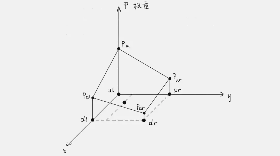
Locate the nearest pixel points with valid RGB information in the four directions of the upper left, upper right, lower left, and lower right, and calculate their distances \(d_{ul}\), \(d_{ur}\), \(d_{dl}\), \(d_{dr}\) to the pixel point to be interpolated. Based on their inverse relationship, assign corresponding weights to the corresponding points.
$$p_{ul}:p_{ur}:p_{dl}:p_{dr}= {1\over d_{ul}}:{1\over d_{ur}}:{1\over d_{dl}}:{1\over d_{dr}}$$

Map the weights to \([0,1]\), then perform weighted assignment for each channel of the points to be interpolated:
$$\begin{bmatrix} R’ \cr G’ \cr B' \end{bmatrix}=p_{ul}\begin{bmatrix} R_{ul} \cr G_{ul} \cr B_{ul} \end{bmatrix}+p_{ur}\begin{bmatrix} R_{ur} \cr G_{ur} \cr B_{ur} \end{bmatrix}+p_{dl}\begin{bmatrix} R_{dl} \cr G_{dl} \cr B_{dl} \end{bmatrix}+p_{dr}\begin{bmatrix} R_{dr} \cr G_{dr} \cr B_{dr} \end{bmatrix}$$
The interpolation of the entire image can be completed by performing the above operations on all the gaps.
Shear#
shear on axis-x \(\begin{bmatrix} x’ \cr y’ \cr 1 \end{bmatrix}=\begin{bmatrix} 1&d_x&0 \cr 0&1&0 \cr 0&0&1 \end{bmatrix}\begin{bmatrix} x \cr y \cr 1 \end{bmatrix}\)
shear on axis-y \(\begin{bmatrix} x’ \cr y’ \cr 1 \end{bmatrix}=\begin{bmatrix} 1&0&0 \cr d_y&1&0 \cr 0&0&1 \end{bmatrix}\begin{bmatrix} x \cr y \cr 1 \end{bmatrix}\)
Mirror#
$$ \begin{bmatrix} x’ \cr y’ \cr 1 \end{bmatrix}= \begin{bmatrix} s_x&0&0 \cr 0&s_y&1 \cr 0&0&1 \end{bmatrix} \begin{bmatrix} x \cr y \cr 1 \end{bmatrix} $$
Convolution#
Principle#
Convolution is the result of multiplying two variables within a certain range and then summing them. The term “convolution” first appeared in signal and linear system theory, where the focus is on the changes that a signal undergoes when passing through a linear system. Due to the common occurrence where the output of a signal at a previous moment affects the output at the current moment, the unit response of the system and the system input are generally used to find the convolution, in order to obtain the output signal of the system.
Of course, this requires the system to be linear and time-invariant). If the convolution variables are the sequences \(x(n)\) and \(h(n)\), the result of the convolution is:
$$ y(n)=\sum_{i=-\infty}^{\infty} x(i) h(n-i)=x(n) * h(n) $$
Image processing convolution#
In image processing, convolution can be used for image filtering, feature extraction, and other processing. Mathematically, the convolution operation can be described using linear algebra methods, which is also a type of affine transformation: a linear transformation of the input vector.
Convolution satisfies the definition of a linear function. If \(f(𝑥)\) satisfies the following two conditions, then \(f(𝑥)\) is said to be a linear function:
$$ \begin{aligned} 𝑓(𝑥1+𝑥2) &= 𝑓(𝑥1)+𝑓(𝑥2) \cr 𝑓(𝑎𝑥) &= 𝑎𝑓(𝑥) \end{aligned} $$
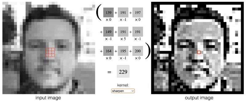
Due to the fact that a digital image is a two-dimensional discrete signal, performing convolution on a digital image actually involves using the convolution kernel to slide across the image, multiplying the pixel values on the image with the corresponding values in the convolution kernel, and then summing all the multiplication results as the pixel value corresponding to the center of the convolution kernel. After sliding across all the pixels, the value of each pixel in the new image is the sum of the products of the pixel values in the original image and the weights of the convolution kernel.
Given an input image \(f(x,y)\) and a convolution kernel \(g(x,y)\), the result of the convolution operation is a new image \(h(x,y)\), where
$$ h(x,y) = ∑∑ f(u,v) * g(x-u, y-v) $$
The convolution kernel \(g(x,y)\) is a small matrix used to perform convolution operations on the input image, and the output image \(h(x,y)\) is a new image obtained by the convolution of \(g(x,y)\) and \(f(x,y)\). Let \(H\) be the result of the convolution operation, which is a new matrix, \(F\) be the matrix representation of the input image, and \(G\) be the matrix representation of the convolution kernel, then the convolution operation can be represented as: \(H = G * F\).

Image Filtering#
The purpose of image filtering is to filter out noise in the image while preserving the image features as much as possible. It is an indispensable operation in image preprocessing, and its filtering effect directly affects the performance of subsequent image recognition, analysis, and other algorithms.
The essence of image filtering is to apply a convolution kernel to the image. Through different convolution kernels, different image processing effects can be achieved, such as edge enhancement, noise removal, and feature extraction.
Here is the translation from Chinese to English:
Some summary of convolutional kernels:
- Convolutional kernels are often matrices with odd numbers of rows and columns, which helps to better locate the center.
- The sum of the kernel elements reflects the brightness of the output. If the sum is 1, the brightness of the convolved image is similar to the original image; if the sum is 0, the convolved image is mostly black, and the brighter parts often represent certain features extracted from the image.
- High-pass filters (HPF) only allow the high-frequency parts (i.e., the parts with drastic changes) of the image to pass through, often used for image sharpening and enhancing the edges of objects in the image.
- Low-pass filters (LPF) only allow the low-frequency parts (i.e., the parts with gentle changes) of the image to pass through, often used for image blurring/smoothing and noise removal. Below are some examples of image filtering methods with their corresponding effect illustrations for reference.
Image mean filtering#
(x’, y’) are the pixel coordinates of the translated image, (x_0, y_0) are the offsets in each direction, and (x, y) are the pixel coordinates of the original image.
The main application of the mean filter is to remove irrelevant details in the image, that is, the pixel regions that are smaller than the size of the filter mask. This is achieved by taking the average of each pixel and its surrounding pixels within a mask (e.g., a 3×3 mask) and then reassigning the value.
$$ Pixel’={1\over9}\times \begin{bmatrix} 1&1&1 \end{bmatrix} \begin{bmatrix} 1\cdot P_{ul} & 1\cdot P_{up} & 1\cdot P_{ur} \cr 1\cdot P_{l} & 1\cdot P & 1\cdot P_{r} \cr 1\cdot P_{dl} & 1\cdot P_{down} & 1\cdot P_{dr} \end{bmatrix} \begin{bmatrix} 1 \cr 1 \cr 1 \end{bmatrix} $$
Image Mean Filtering Example


Laplace Image Enhancement#
Principle: The Laplace operator can approximate the second-order derivative of an image, which has rotational invariance, meaning it can detect edges in all directions.
The Laplace operator
$$ \nabla^2f={\partial^2f\over\partial x^2}+{\partial^2f\over\partial y^2} $$
It includes:
$$ \begin{aligned} {\partial^2f\over\partial x^2}=f(x+1,y)+f(x-1,y)-2f(x,y) \cr {\partial^2f\over\partial y^2}=f(x,y+1)+f(x,y-1)-2f(x,y) \end{aligned} $$
After incorporating the diagonal direction into the discussion
$$ \begin{aligned} {\nabla^2f}=[f(x-1,y-1)+f(x,y-1)+f(x-1,y)+f(x+1,y)+\cr f(x-1,y+1)+f(x,y+1)+f(x+1, y+1)]-8f(x,y) \end{aligned} $$
Due to the sudden change in pixel information values at the edges, i.e., the first-order derivative has a local maximum, this feature can be used to further calculate the second-order derivative equal to 0, and the above formula is the result of discretizing the second-order derivative. By using the Laplacian operator, the parts of the image where the information value (a certain RGB channel value) changes abruptly can be extracted, and this part is the edge of the image. Finally, by overlaying this with the original image, an edge-enhanced (sharpened) image is obtained. (Where \(Pixel’\) is the pixel coordinate of the transformed image)
- Filtering:
$$ Pixel’={1\over9} \times \begin{bmatrix} 1&1&1 \end{bmatrix} \begin{bmatrix} 1\cdot P_{ul} & 1\cdot P_{up} & 1\cdot P_{ur} \cr 1\cdot P_{l} & -8\cdot P & 1\cdot P_{r} \cr 1\cdot P_{dl} & 1\cdot P_{down} & 1\cdot P_{dr} \end{bmatrix} \begin{bmatrix} 1 \cr 1 \cr 1 \end{bmatrix} $$
- Superimpose:
$$ Pixel’’=Pixel - Pixel' $$
Laplacian Image Enhancement Example


